Here, we address the pragmatic question: What Urazori (reverse curve) shapes result in a chosen braced shape? Anticipating the actual construction of yumi, we require a quantitative answer. Traditional yumishi laminate an initially extreme Urazori shape, and the final Urazori shape is adjusted by heat aided bending. We anticipate using modern materials. In particular, there may be carbon laminations between the bamboo back and belly laminations and the core. Such a construction does not have the malleability of a traditional take-yumi, made of all natural materials. The correct Urazori shape has to be achieved at the outset. Little adjustment is possible. The phrasing of the initial question suggests that there may be more than one Urazori shape corresponding to the correct braced shape. This is true and we will come to that. We begin with a simplified review of how forces applied to the ends of an elastic beam bend it. Of course we have in mind the yumi as the beam, and the string tensions due to the tsuru are the forces.
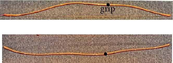
Figure 1 compares the braced shape with the unbraced Urazori (reverse curve) shape of a Don Symanski yumi. We’ve seen this yumi before while investigating the aesthetics of yumi shape. (Figures 5 and 6 of the page “Geometry, Aesthetics and the Yumi.”)
Fig. 1: Braced and unbraced shapes.
Curvature and bending
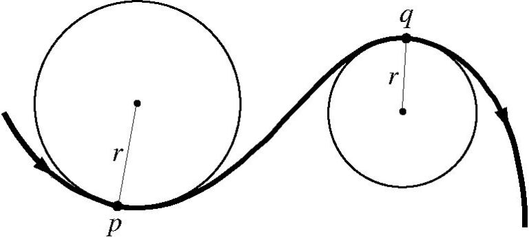
The physics of bending in a plane singles out the geometric property called “curvature.” Figure 2 shows a section of a smooth plane curve. We assign a definite direction or “orientation” of the curve as indicated by the arrows in Fig. 2. At any point p along the curve, there is a circle which most closely “kisses” it. Imagine the curve as a trail, and you are walking along it and looking in the direction indicated by its orientation. If at point p, you see the portion of circle near you to your left, the curvature at p is defined to be the reciprocal of the circle’s radius r,
κ = 1/r.
If the nearby portion of circle is to your right, like at point q, the curvature is the negative of the reciprocal,
κ = -1/r.
Look at the curve in Fig. 2 from above. At the point p where the curvature is positive, the curve looks concave. At the point q where the curvature is negative, it looks convex. In describing yumi shapes, we’ll refer to visualizations like the top panel of Fig. 1: The tsuru is horizontal and the yumi is “above” it. Then yumi segments with negative curvature are concave when seen from the above (or the back) and segments with positive curvature are convex.
Having defined curvature of an elastic beam in a plane, we define “bending” at a material point along the beam as the change in curvature induced by forces acting on it.
Fig. 2: The definition of curvature.
Bending and the torque identity
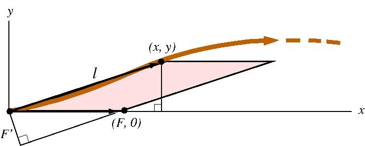
Bending is quantified by the “torque identity.” In Fig. 3, the elastic beam is represented by the brown curve, oriented from left to right. You can think of it as a portion of yumi limb below the grip. The tsuru extends from the tip (0, 0) along the x axis to the right, exerting a horizontal tension force F. What is the change Δ κ of curvature at a material point (x, y) along the beam? Intuitively, a force applied at the end (0, 0) is more effective at bending if it is perpendicular to the displacement from (0, 0) to (x, y). In Fig. 3, this displacement is represented by an arrow, and l denotes its length. F’ denotes the component of the force perpendicular to this displacement. The change of curvature at the material point (x, y) along the limb is directly proportional to F’: We have the “torque identity,”
μ Δ κ = – l F’.
The positive number μ is called the “bending stiffness” of the beam at the material point (x, y). The right hand side -lF’ is called the “torque exerted by the horizontal force F on the beam at (x, y).” Geometrically, the product lF’ is the area of the pink parallelogram in Fig. 3. This area is also given by Fy, so we have the alternative form of the torque identity,
μ Δ κ = -yF.
This form of the torque identity informs the relationship between braced and Urazori shapes.
This simple description of the torque identity idealizes the yumi as an elastic material curve with no thickness. Practical design calculations are improved by acknowledging the actual thickness of a physical yumi. In a simple model, we imagine that the mass and elasticity of the yumi are concentrated along a center line between the back and belly. The tips of this center line curve lie above the ends of the tsuru by half of the limb thickness. The elevation profile is taken relative to the tsuru.
Fig. 3: Geometry of the torque identity.
Unbraced Urazori shape determined from the braced shape
For a given braced yumi, the string tension F has some definite value. The elevation y and stiffness μ are definite functions of length along the yumi, called “elevation and stiffness profiles.” Given the tsuru tension and elevation and stiffness profiles, the torque identity determines the curvature changes Δ κ along along the length of the yumi when we brace it. If the braced shape is prescribed, then so is the braced curvature κ B. We may now calculate the Urazori curvature profile from
κU = κB – Δ κ.
Finally, we determine the Urazori shape from its curvature profile. We now proceed with the operational details.
Spline approximations of yumi shapes
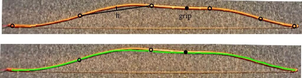
In the article “Geometry, Aesthetics and the Yumi,” we characterized the five curves of a yumi by their lengths and depths. In the top panel of Fig. 4, the hollow dots represent curve endpoints which are also inflection points where the curvature vanishes. The depth of a curve is the perpendicular distance of the curve’s midpoint from the chord line connecting its endpoints. In Fig. 4, we’ve drawn the chord of the second curve from the top, and indicted its depth h. Recall that the depth is positive for curves which are convex when seen from the back, and negative if concave. Given the length and depth of any curve, we approximate the shape between its endpoints by a mathematically simple curve, generally called a “spline.” The splines we use are very close to half periods of a sine wave, so we call them “trigonometric splines.” The “spline approximation” to the yumi shape is obtained by joining the splines end to end in the correct order. In the bottom panel of Fig. 4, the green curve is the spline approximation based on the measured curve lengths and depths of the Yonsun yumi in Fig. 4. The spline of any given curve is symmetric about its midpoint. The second curve of the actual yumi is not symmetric about its midpoint, with its right side bulging above the spline curve. As we shall see, there is some weakness there.
Fig. 4: Top panel: The hollow dots are endpoints of the five curves of the Don Symanski Yonsun yumi in Fig. 1. We visualize the depth h of the second curve as the elevation of its midpoint above its chord line. Bottom panel: Spline approximation to the shape of the yumi.
The stiffness profile
Intuitively, the stiffness of a yumi is the greatest at the grip and decreases as we move towards either tip. What do stiffness profiles of actual yumi look like? We get an idea by estimating the stiffness profile of the Don Symanski yumi depicted in Fig. 1. The estimated stiffness profile is deduced from suitable measurements and the torque identity: We measure the tsuru tension of the braced yumi. By comparing shapes of the braced and unbraced yumi, we deduce the curvature change profile induced by bracing. Knowing the tsuru tension F, the elevation profile y of the braced yumi and the curvature change profile Δ κ induced by bracing, we estimate the stiffness profile by “solving” the torque identity for the stiffness profile μ. Details are spelled out in the article “Shape of the Yumi” linked to this page.
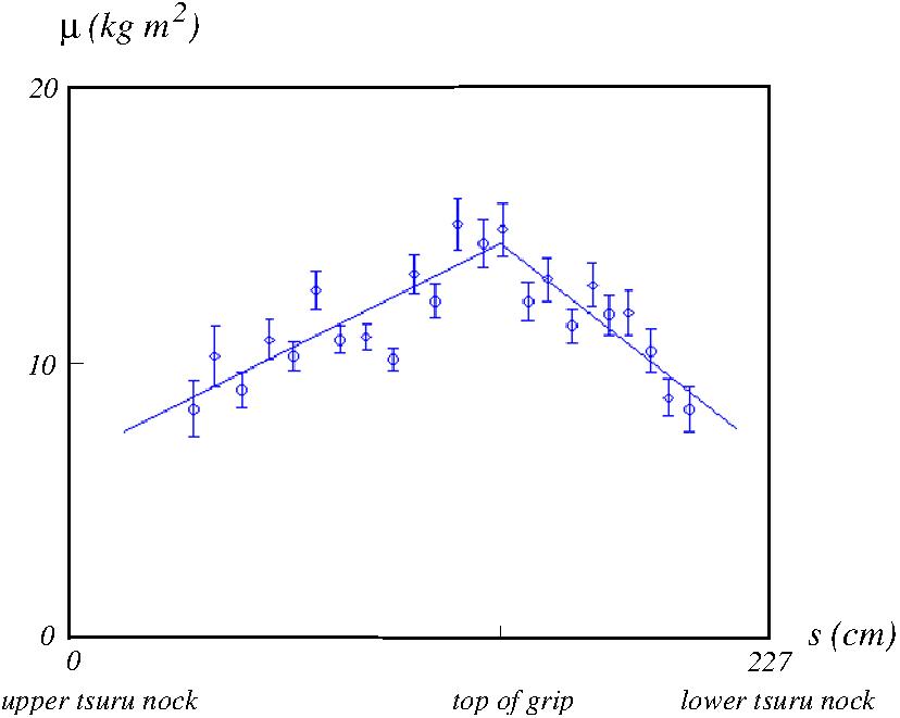
The horizontal axis of the graph in Fig. 5 is length s along the yumi measured from the upper tsuru nock in centimeters. The vertical axis is the stiffness μ in kilograms meters squared (kg m2). The physical units kg m2 of stiffness is informed by the torque identity. In the right hand side, the tsuru tension F is measured in kilograms, and the braced elevation y in meters, so the right hand side has physical units of kilograms times meters. In the left hand side, curvature and hence the change Δ κ in curvature is measured in inverse meters. The balance of physical units in the torque identity indicates that the physical units of stiffness are kilograms times meters squared. The discrete data points are obtained by measurements of braced elevation y and curvature change Δ κ induced by bracing at distinct material points along the yumi. The diamonds correspond to belly or back nodes, the circles to midpoints between adjacent back and belly nodes. You would expect the stiffness at nodes to be a bit higher than between nodes, and the data is mostly consistent with this. Recall that the right side of the second curve from the top appears to be weak, because it bulges above the spline approximation in Fig. 4. We can see the weak section in the fifth data point of Fig. 5 above the grip.
Underlying the scatter in the data, we see decreases in stiffness away from the grip which is roughly proportional to distance from the grip. The stiffness near the tips is roughly half of the stiffness at the grip. In our design of the Urazori shape, we assume this simple structure of the stiffness profile.
Fig. 5: Measured stiffness profile of the Don Symanski yumi.
A test case
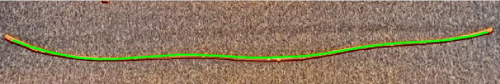
We have a spline approximation to the braced shape of the Don Symanski Yonsun, which yields collateral approximations to the braced elevation and curvature profiles. We adopt the piecewise linear approximation to the stiffness profile, as in the graph of Fig. 5. The braced tsuru tension is measured, F = 32.05 kg. This is all the information we need to calculate an approximation to the unbraced curvature profile from the torque identity. From the unbraced curvature profile, we finally compute the predicted Urazori shape. In Fig. 6, we’ve reproduced the bottom photograph of the actual Urazori shape from Fig. 1. The super-positioned green curve is the predicted Urazori shape from the torque identity calculation.
Fig. 6: The green curve is the computed Urazori shape super-positioned over the photograph of the actual Urazori shape of the Don Symanski Yonsun.
The multiplicity of Urazori shapes
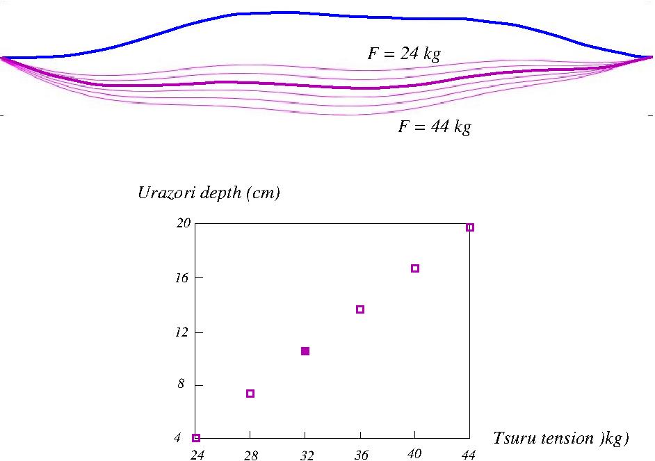
The blue curve in the top panel of Fig. 7 is the spline approximation to the shape of the braced Don Symanski Yonsun. The magenta curves are computed Urazori shapes corresponding to a sequence tsuru tensions between 24 kg and 44 kg. We highlight the Urazori shape whose brace tension is very near the measured value, 30.05 kg. We define the Urazori depth as the greatest perpendicular displacement of the Urazori shape curve from the chord line between its tips. The second panel of Fig. 7 plots the Urazori depth versus the brace tension.
Fig. 7: Top panel: Urazori shapes (magenta curves) corresponding to the braced shape of the Don Symanski Yonsun (blue curve). Bottom panel: The Urazori depth increases with the tsuru tension.
A proposal for the yumishi
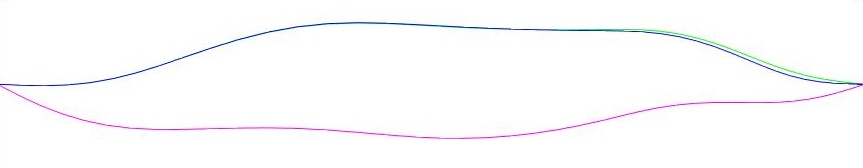
In Fig. 8, the blue curve is the original “mirror symmetry” shape, which is nearly tangent to the tsuru at the lower tip. The green curve is a “broken mirror symmetry” shape which opens up the angle between the yumi shape and the tsuru at the lower tip. The magenta curve is the “broken mirror symmetry” Urazori shape whose depth is 15 cm. The layup of this shape in the shop is described in the page “Yumi Making Re-examined.”